第一篇我们讲了matplot画图的基本要素,第二篇讲matplot若干个常见的基础图的画图操作。最后一篇我们讲一下matplot画图中可能会用到的几个高级用法。
Subplot 多图合一
matplotlib 是可以组合许多的小图, 放在一张大图里面显示的. 使用到的方法叫作 subplot.
均匀分布
1 | import matplotlib.pyplot as plt |
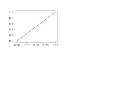
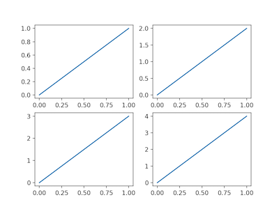
将这四个区域都填满:
1 | plt.figure() |
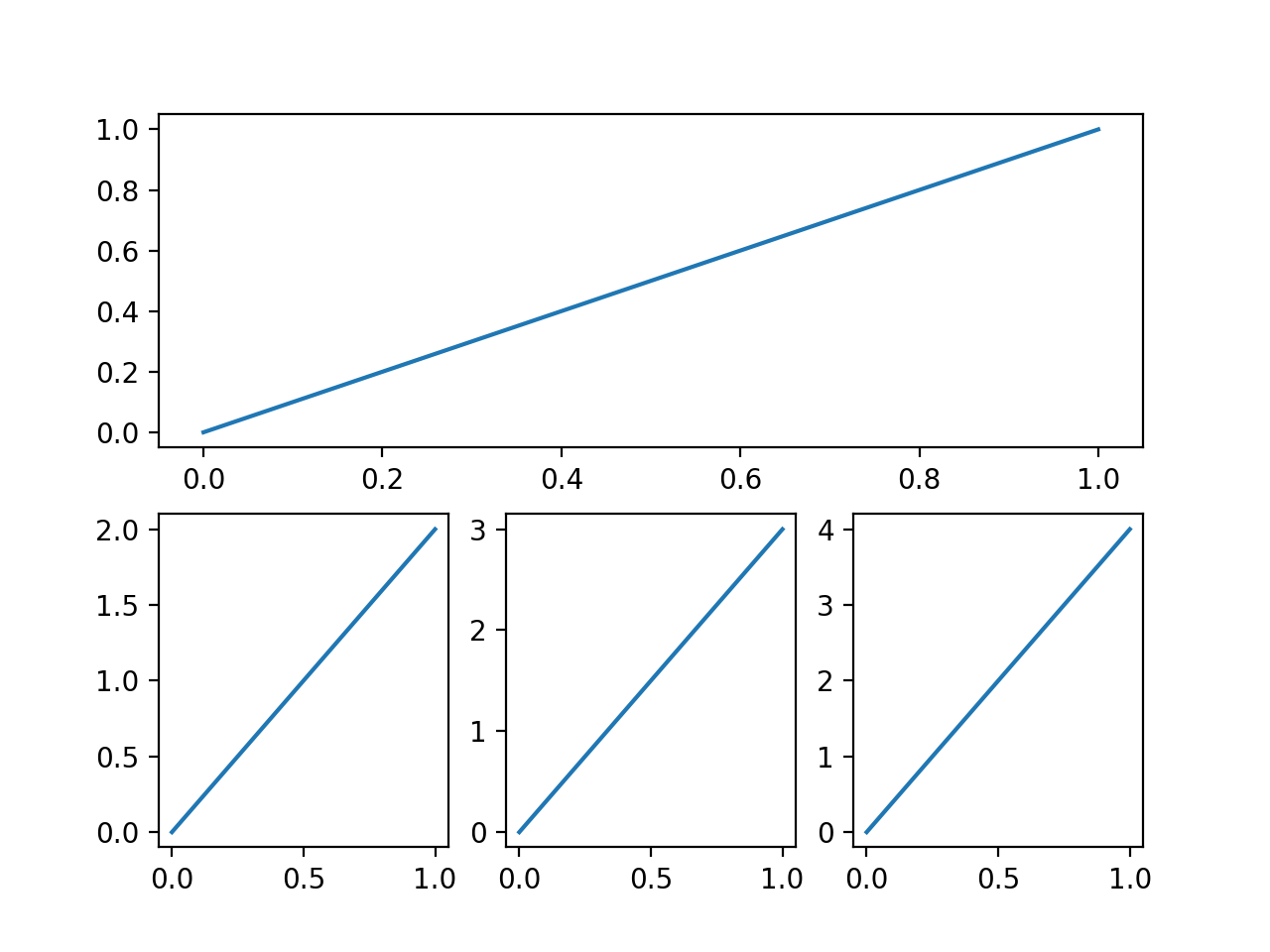
非均匀分布
1 | plt.subplot(2, 1, 1) # 两行一列 |
分格
subplot2grid()方法
1 | import matplotlib.pyplot as plt |

gridspec
导入matplotlib.gridspec模块
1 |
|

subplots()
借助subplots()方法,我们也可以分格显示图像
1 | f, ((ax11, ax12), (ax13, ax14)) = plt.subplots(2, 2, sharex=True, sharey=True) |

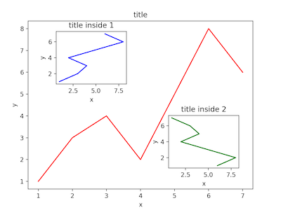
plot in plot 图中图
matplot支持我们在同一个figure里面,画多个图。也就是图中图。
先画一个大图
1 | import matplotlib.pyplot as plt |
接着我们画左上角的小图
1 | left, bottom, width, height = 0.2, 0.6, 0.25, 0.25 |
然后是右下角的小图
1 | plt.axes([0.6, 0.2, 0.25, 0.25]) |
Animation 动画
matplot支持我们展示动画,首先我们需要导入animation模块
1 | import matplotlib.pyplot as plt |
接下来我们定义一个0~2π内的正弦曲线

1 | fig, ax = plt.subplots() |
1 | # 定义动画 |
保存为视频
1 | ani.save('basic_animation.mp4', fps=30, extra_args=['-vcodec', 'libx264']) |
当然,如果报错的话,记得安装一下ffmpeg或者mencoder,例如mac下:
1 | brew install ffmpeg |
保存为gif图
1 | ani.save('basic_animation.gif', writer='imagemagick', fps=60) |